Thank you! Your submission has been received!

Oops! Something went wrong while submitting the form.

CIFAR-10

Please note that Squint Vision Studio defines a “Datasource” as a collection of data used to train and evaluate a model (e.g. CIFAR10) and a “Dataset” as a datasource descriptor created in Squint Vision Studio to manage the datasource.

CIFAR-10 Dataset Classification

This guide walks you through a complete workflow in Squint Vision Studio using the CIFAR-10 datasource; a collection of natural images that are commonly used to train machine learning and computer vision algorithms. You will be guided through the process of setting up a project, creating a CIFAR-10 dataset from the CIFAR-10 datasource, importing a model, and leveraging Squint Vision Studio's tools to thoroughly evaluate, interpret, and monitor your model's performance.

The following sections will walk you through how to use Squint Vision Studio, so it is expected that you have the Studio open and have obtained a valid license.

Project Setup: CIFAR-10

1. Project Setup

Creating a Project

Navigate to the Project tab.
Click Load to open an existing project or click the + icon next to Manage projects to create a new one.
Name your project (e.g., CIFAR-10 Classification) and optionally add a description.
Click Save.

2. Dataset: CIFAR-10

Dataset: CIFAR-10

Preparing the Datasource

The CIFAR-10 datasource should be placed in the SquintVolume/DataSources directory and structured as follows:

A top-level folder should be created with the datasource name (e.g. CIFAR-10).
Inside, create two subfolders: train and test.
Each of these contains 10 subfolders, one for each class:

Airplane
Automobile
Bird
Cat
Deer
Dog
Frog
Horse
Ship
Truck

Each class folder should contain the corresponding image files.

Example code to create a CIFAR-10 datasource

TensorFlow provides the CIFAR-10 datasource as a tuple of NumPy arrays, where the images and labels are stored separately for training and testing. Each image is a 32×32 color image represented as a NumPy array, and each label corresponds to one of 10 object classes. This format is convenient for training models directly in code, but it does not match the folder-based structure required by Squint Vision Studio. Squint Vision Studio expects the data to be organized into directories by class label, with each image saved as an individual file. Therefore, we need to convert the datasource from its in-memory array format into a structured directory format. We provide the following code as an example of how a datasource can be converted from a numpy-array dictionary format to a directory structure where the labels can be inferred from the folder names. You can use this code to create your own CIFAR-10 datasource, or to create a datasource out of your own real-world data

Copied!

import os
import numpy as np
from tensorflow.keras.datasets import cifar10
from PIL import Image

# Define the base directory
base_dir = 'SquintVolume/DataSources/CIFAR-10'

# Define subdirectories
splits = ['train', 'test']
classes = [str(i) for i in range(10)]

# Create directory structure
for split in splits:
    for cls in classes:
        os.makedirs(os.path.join(base_dir, split, cls), exist_ok=True)

# Load CIFAR-10 dataset
(x_train, y_train), (x_test, y_test) = cifar10.load_data()

# Helper function to save images
def save_images(images, labels, split):
    for idx, (img, label) in enumerate(zip(images, labels)):
        img = Image.fromarray(img)
        img_path = os.path.join(base_dir, split, str(label), f'{idx}.png')
        img.save(img_path)

# Save training and test images
save_images(x_train, y_train, 'train')
save_images(x_test, y_test, 'test')

print("CIFAR-10 datasource has been saved in the required folder structure.")

Creating the Dataset

In the Studio, navigate to Data ⇀ Load.
Click the + icon to create a new dataset.
Select the CIFAR-10 data source.
Apply data preprocessing as illustrated in the image below.

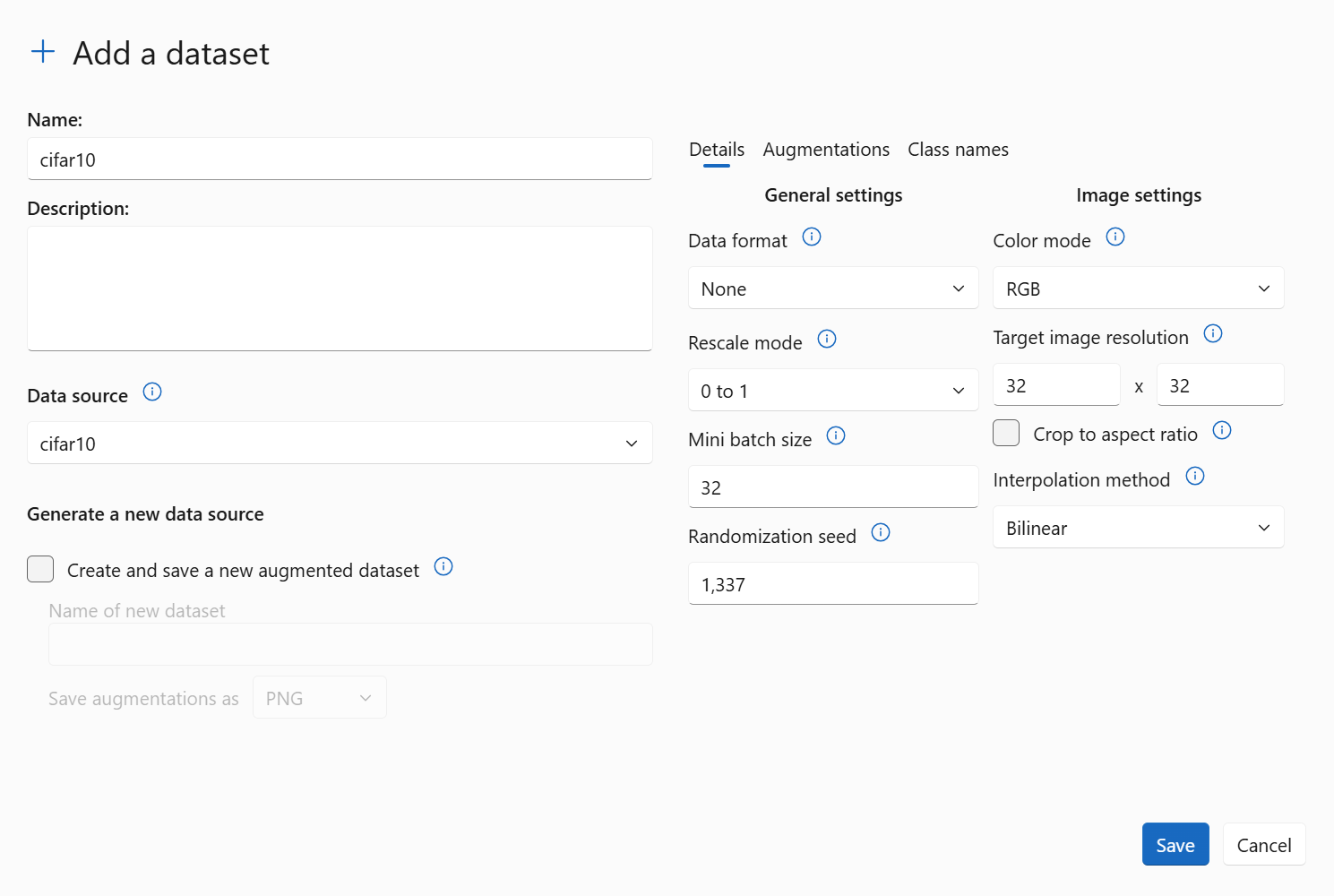
We use a target image resolution of 32×32 pixels because that is the native size of the images in the CIFAR-10 datasource, and it matches the expected input size of our model (which we will define below). CIFAR-10 consists of color images of various object classes, and each image has three channels (RGB). Therefore, we chose the color mode as RGB.
To prepare the data for training, we normalize the pixel values to the range [0, 1] by dividing each value by 255. This normalization helped improve model performance and training stability in our experiments. As a result, we selected the rescale mode of 0 to 1. Note that once you are working with your own datasource and model, the settings you specify when creating the dataset should match your own model/data expectations.
The mini batch size should be set to whatever batch size you use while training your model on the datasource. In this case we left the default setting of 32 as that’s the same batch size we use while training our model (see below).

Save the dataset.

Exploring the CIFAR-10 Dataset

Navigate to Data ⇀ View – Browse CIFAR-10 Images Using the Image Carousel

The View feature provides an interactive image carousel that lets you visually inspect the images in the CIFAR-10 dataset.

Scroll through images by category to verify data quality and labeling.
Confirm that images are correctly grouped by class.
Identify any anomalies, such as misclassified or low-quality images.

This tool is especially useful for validating the dataset before training or evaluating models.

Navigate to Data ⇀ Metrics – View per-class sample distribution and dataset statistics

The Metrics feature offers a statistical overview of the CIFAR-10 dataset, helping you understand its structure and balance.

View the number of samples per class in both training and test sets.
Detect any class imbalances that could affect model performance and bias
Review the overall dataset size and class diversity.

These insights are essential for diagnosing potential biases and ensuring the dataset is well-prepared for training and evaluation.

Navigate to Data ⇀ Histogram – Analyze per-class pixel intensity distributions

The Histogram feature visualizes the pixel intensity distributions for each class in the CIFAR-10 dataset.

Analyze brightness and contrast patterns across different categories.
Detect inconsistencies or anomalies in image quality.
Compare visual characteristics between classes to assess uniformity.

This tool helps ensure that the dataset is visually consistent and suitable for model training.

3. Model: CIFAR-10 Classifier

Model: CIFAR-10 Classifier

Uploading the trained Model

Navigate to the Model ⇀ Load page.
Load a previously added model, or click on the + icon to add a vision model trained on CIFAR-10 to the studio
Create a model descriptor and link it to your project.

Note: The model must be trained before uploading. Squint Vision Studio is not intended for training models; it is designed for deploying and analyzing already-trained models. Ensure your model is trained externally and then uploaded to the studio.

Below is an example of how you can train a Convolutional Neural Network (CNN) model on the CIFAR-10 datasource before uploading it to Squint Vision Studio:

Structure of the CNN Model

Copied!

from tensorflow 
import keras from tensorflow.keras.layers 
import Conv2D, BatchNormalization, MaxPooling2D, Dropout, Flatten, Dense

# Define the input shape for CIFAR-10 images
input_layer = keras.Input(shape=(32, 32, 3))

# Block 1: Convolutional layers with batch normalization and dropout
x = Conv2D(32, (3, 3), activation='relu', padding='same')(input_layer)
x = BatchNormalization()(x)
x = Conv2D(32, (3, 3), activation='relu', padding='same')(x)
x = BatchNormalization()(x)
x = MaxPooling2D(pool_size=(2, 2))(x)
x = Dropout(0.3)(x)

# Block 2
x = Conv2D(64, (3, 3), activation='relu', padding='same')(x)
x = BatchNormalization()(x)
x = Conv2D(64, (3, 3), activation='relu', padding='same')(x)
x = BatchNormalization()(x)
x = MaxPooling2D(pool_size=(2, 2))(x)
x = Dropout(0.3)(x)

# Block 3
x = Conv2D(128, (3, 3), activation='relu', padding='same')(x)
x = BatchNormalization()(x)
x = Conv2D(128, (3, 3), activation='relu', padding='same')(x)
x = BatchNormalization()(x)
x = MaxPooling2D(pool_size=(2, 2))(x)
x = Dropout(0.3)(x)

# Block 4
x = Conv2D(128, (3, 3), activation='relu', padding='same')(x)
x = BatchNormalization()(x)

# Flatten and fully connected layers
x = Flatten()(x)
x = Dense(1024, activation='relu')(x)
x = BatchNormalization()(x)
x = Dropout(0.3)(x)

x = Dense(512, activation='relu')(x)
x = BatchNormalization()(x)
x = Dropout(0.3)(x)

# Output layer for 10 classes
output_layer = Dense(10, activation='softmax')(x)

# Construct the model
model = keras.Model(inputs=input_layer, outputs=output_layer)

Training the CNN Model

Copied!

# Compile the model
model.compile(
    loss='categorical_crossentropy',
    optimizer='adam',
    metrics=['accuracy']
)

# Train the model
history = model.fit(
    X_train, y_train,
    epochs=50,
    batch_size=32,
    verbose=1,
    shuffle=True,
    validation_split=0.5
)

# Save the trained model
model.save('cifar10_model.keras')

Explore the model and capture intermediate representations

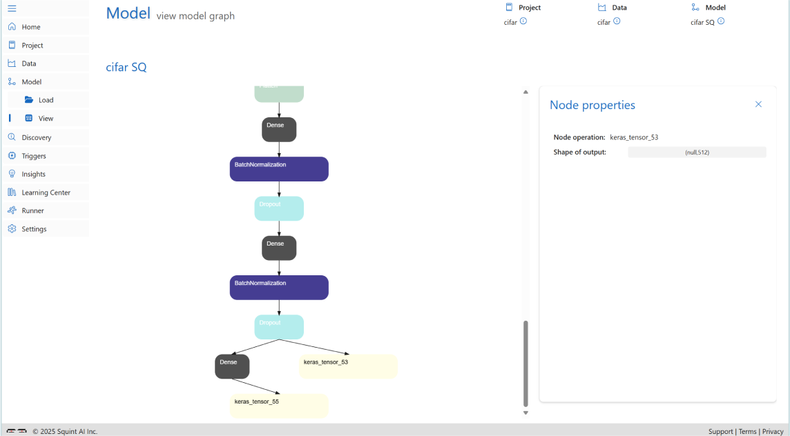
Use the View feature to inspect the model graph.
Click on model nodes to view layer details.
Select a node and click Generate Model to create a squinting model that captures intermediate outputs. A squinting model is a modified version of your original model designed to capture and output intermediate activations from specific layers during inference. This step is crucial as we will need to evaluate how your model sees the data (e.g. by capturing the embeddings of a layer deep in the model) before we can proceed to create a discovery.
Once you click “Generate Model” from a model node, navigate back to the Model ⇀ Load page and load the newly created squinting (“SQ”) model. In this project, we selected the final Dropout layer as the feature extraction layer, which has an output shape of (None, 512), as shown in the image below. This indicates that we are capturing the output from this layer to analyze how the model processes data at that stage, where the layer produces 512 features per input sample.

4. Discovery: Evaluating the CIFAR-10 Model

Discovery: Evaluating the CIFAR-10 Model

Creating a Discovery

Navigate to the Discovery ⇀ Load page.
Click on the + icon to create a new discovery.
The model will run inference on the CIFAR-10 dataset and generate performance metrics.

Discovery ⇀ Metrics

Analyze mistake distributions across classes for both training and testing sets. The image below illustrates how errors are distributed per class, helping to identify which categories are more prone to misclassification.

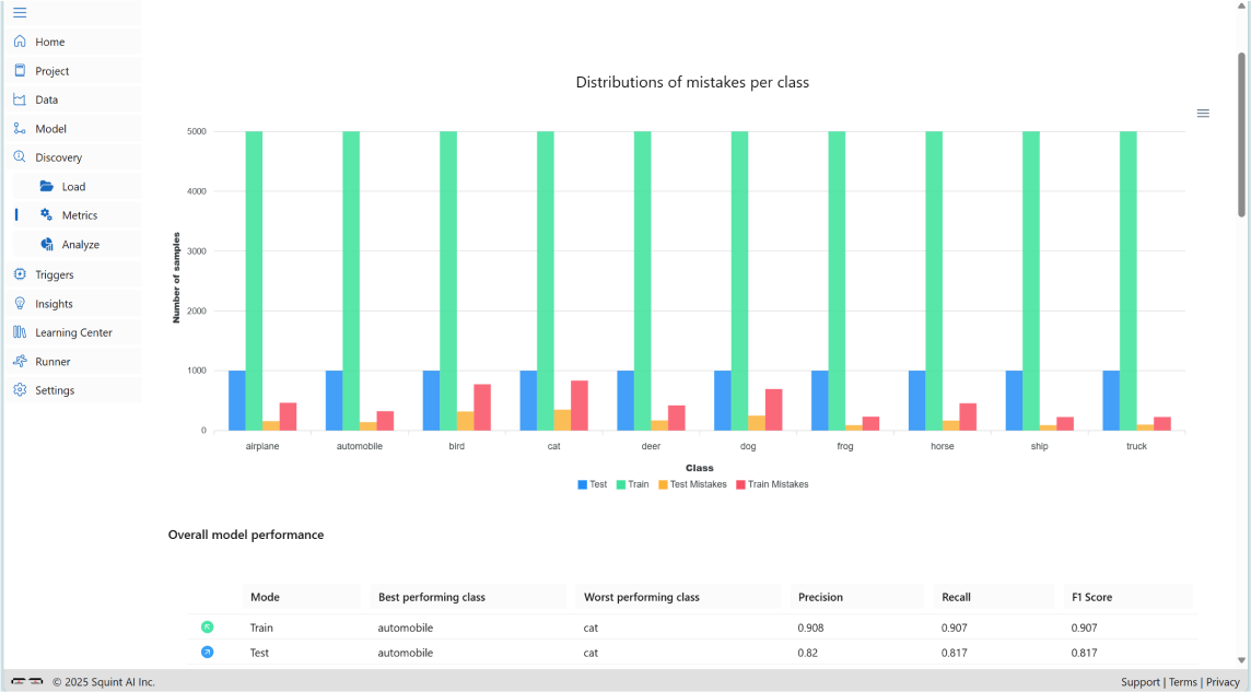
Evaluate overall model performance on training and testing sets. Identify the best and worst performing classes (e.g., class automobile performs best, class cat performs worst).
Examine per-class performance metrics, including accuracy, F1 scores, and error distributions for both training and testing sets.
Inspect confusion matrices for training and testing sets to identify commonly misclassified classes (e.g., frequent confusion between classes cat and dog).
View dataset information used in this discovery, including dataset details and any augmentations applied during preprocessing or training.

Discovery ⇀ Analyze

Explore the embedding space of the model (based on the layer selected when creating the squinting model) using the Cognitive Atlas. In the Cognitive Atlas you can explore the relationships your model sees in the data by analyzing scatter plots for both training and testing data (select “train” or “test” sunder Image Source). You can analyze the model’s perception for all classes at once, or by selecting specific classes using the “class filter” control; by default, all classes are shown.
Below is a cognitive atlas generated for this project, illustrating the embedding space on the CIFAR-10 training data:

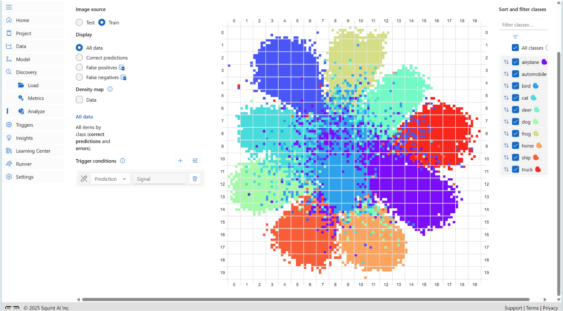
Analyze the embedding space by selecting different Display options to view all data points, correct predictions, false positives, and false negatives. You can also filter by class using the selection bar on the right (default shows all classes).
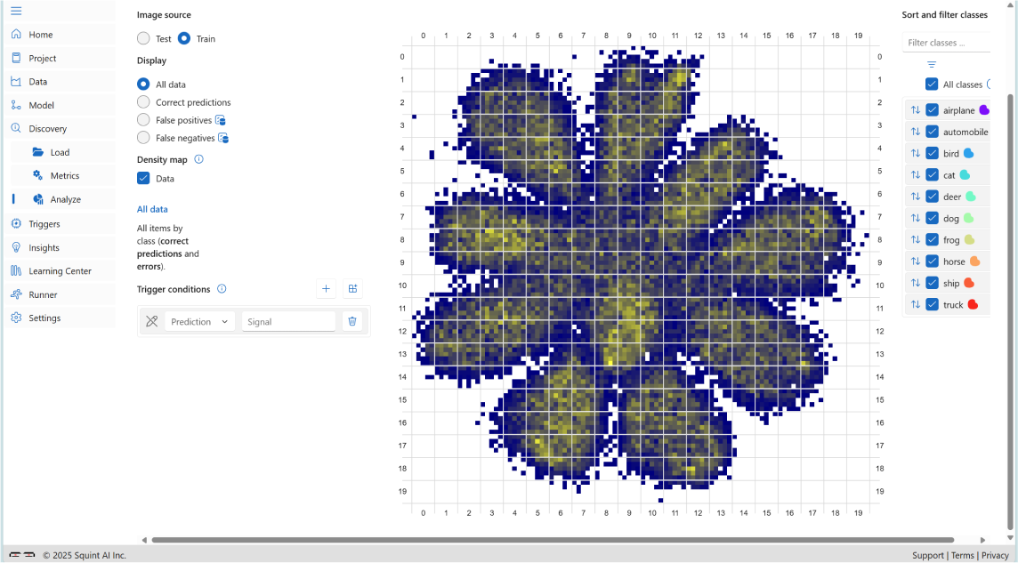
The image below shows false positive errors across all classes in the CIFAR-10 training data, visualized on the scatter plot.

As shown in the image, most errors are concentrated near the edges of the clusters in the embedding space. These boundary areas, which we refer to as ambiguous regions, represent zones where the model struggles to distinguish between classes. In these regions, the feature representations of different classes overlap or are very close, making it difficult for the model to make confident predictions. As a result, predictions in ambiguous regions are less reliable and more prone to error.
In contrast, the central areas of the clusters referred to as trusted regions, are where the data points are more densely packed and clearly separated from other classes. These regions reflect high-confidence zones where the model consistently makes correct predictions.
The lack of errors in these areas suggests that the model has learned strong, discriminative features for those examples, making its predictions more dependable.
Understanding the distribution of errors in the embedding space helps in diagnosing model behavior, identifying areas of uncertainty, and guiding improvements such as targeted data augmentation or model calibration.

Use the DensityMap option in Squint Vision Studio to visualize the distribution of data in the embedding space.
When All Data is selected in the Display menu, the DensityMap shows the overall data distribution. It highlights areas with the highest concentration of data points. The image below shows the DensityMap for the data on the CIFAR-10 training set. As you can see in the image, the densest regions are located at the center of the clusters, while the edges represent areas of lower density.

When False Positive or False Negative is selected in the Display menu, it highlights areas with the highest concentration of mistakes. This helps identify problematic regions or cells in the embedding space. By focusing on these areas; such as setting triggers or targeted improvements; you can enhance model performance more effectively. The image below shows the DensityMap for Incorrect Predictions on the CIFAR-10 training set:

Interactively explore ambiguous regions in the embedding space by clicking on cells located near the edges of clusters in the scatter plot. These edge cells often represent areas where the model is uncertain, leading to a higher likelihood of misclassifications. When you click on a cell, you can view detailed cell statistics and browse the image gallery of similar embeddings within that region.
The image below shows cell statistics for a selected cell in an ambiguous region of the CIFAR-10 training set:

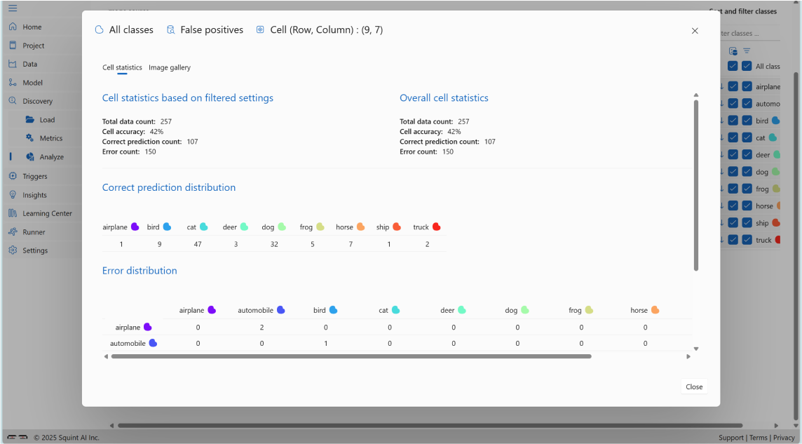
Cell Statistics

These represent the full statistics for the cell, regardless of filters:

Total Data Count: 257
Cell Accuracy: 42%
Correct Prediction Count: 107
Error Count: 150

Correct Prediction Distribution

This breakdown shows how many correct predictions were made per class within the cell:

Airplane: 1
Automobile: 0
Bird: 9
Cat: 47
Deer: 3
Dog: 32
Frog: 5
Horse: 7
Ship: 1
Truck: 2

Error Distribution

This breakdown shows the number of misclassifications per class:

Airplane: 2
Automobile: 1
Bird: 14
Cat: 68
Deer: 8
Dog: 41
Frog: 9
Horse: 4
Ship: 3
Truck: 0

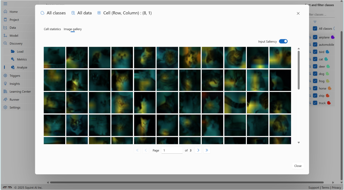
The image below shows image gallery for a selected cell in an ambiguous region of the CIFAR-10 training set:

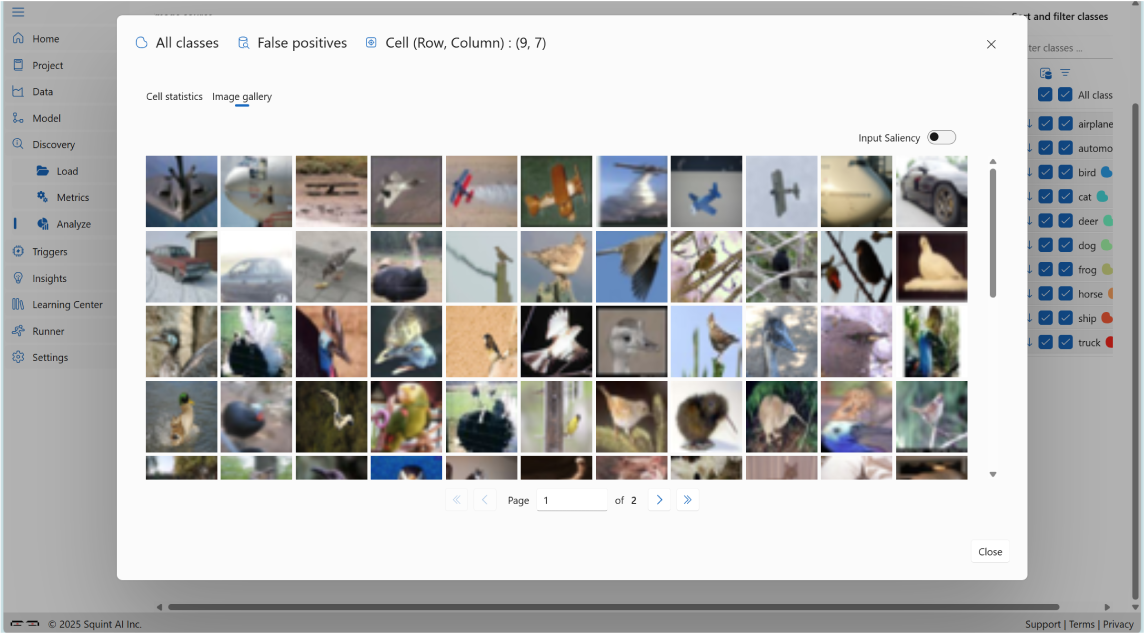
As you can see, the images are ambiguous and not clearly recognizable.
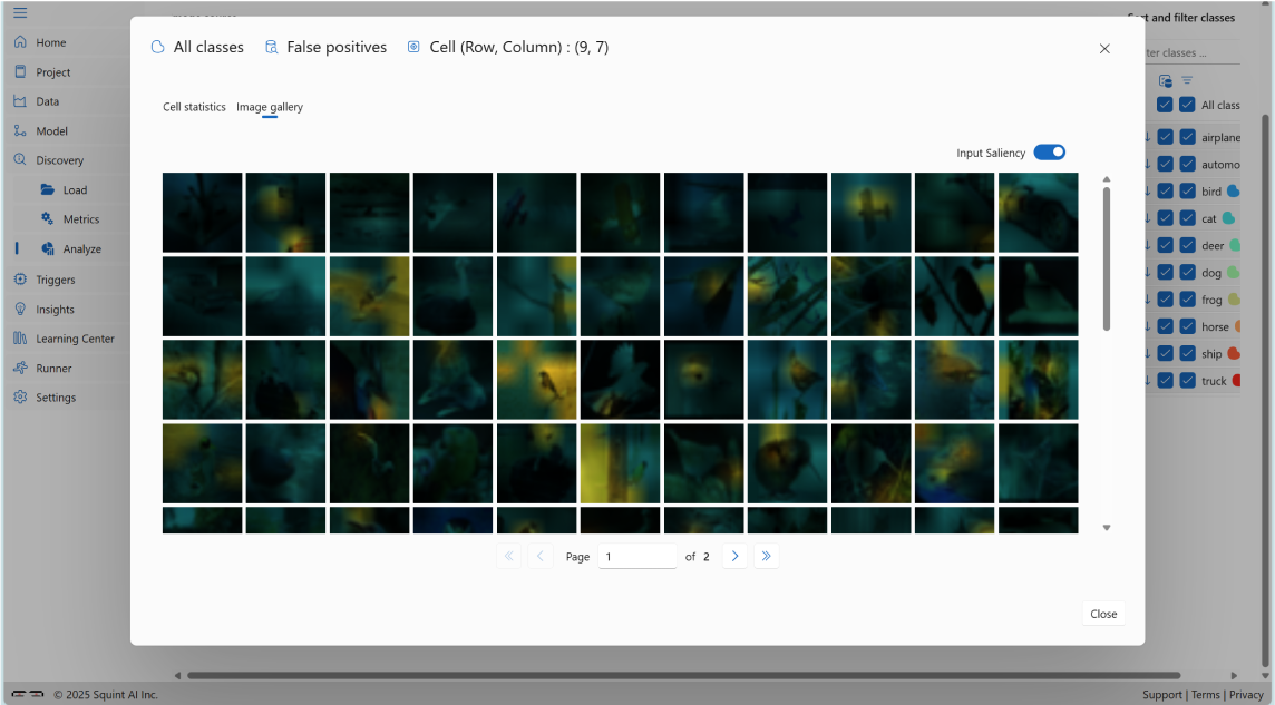
You can also select the Input Saliency option (top-right corner of the image gallery) to highlight which parts of the images influenced the model's predictions, as shown below:

Interactively explore trusted regions in the embedding space by clicking on cells located near the center of clusters, typically represent areas where the model is trustworthy, resulting in fewer misclassifications. Clicking on a cell reveals cell statistics and an image gallery of consistent embeddings.The image below shows cell statistics for a selected cell in trusted region of the class cat of the CIFAR-10 training set:

Cell Statistics:

Total Data Count: 205
Cell Accuracy: 100%
Correct Prediction Count: 205
Error Count: 0

Correct Prediction Distribution:

Class cat: 205

The image below shows image gallery for a selected cell in the trusted region of the class cat of the CIFAR-10 training set:

As you can see, the images are clear and consistent, making them easier to recognize.
You can also select the Input Saliency option (top-right corner of the image gallery) to highlight which parts of the images influenced the model's predictions, as shown below:

5. Trigger: Monitoring CIFAR-10 Predictions

Trigger: Monitoring CIFAR-10 Predictions

A trigger is a set of conditions that a user can design using the Cognitive Atlas to monitor the predictions of a model at runtime.

Note: that a premium license is required to access the Trigger feature.

Creating a Trigger

Go to Discovery ⇀ Analyze page.
Click the + button in front of Trigger conditions to create a new trigger.
Select cells in the embedding space where the model shows uncertainty or frequent misclassifications (e.g., where categories like cat and dog overlap).
These selected cells will appear in the create Triggers dialog.
Define the trigger condition (e.g., "If the model predicts cat and the input falls in the cell (6, 12), fire alert ‘Confusion between cat and dog’").
Save the trigger.

Exporting a Trigger

Navigate to the Trigger ⇀ Export page.
View the trigger's conditions as diagrams showing:

The monitored cells for each prediction.
The alert value returned when the condition is met.

Exporting a trigger generates a runtime watchdog.
The watchdog can be integrated into your application using the Squint Watchdog API to monitor predictions and flag ambiguous or out of distribution inputs in real time.

Example: Creating a Trigger for Class Cat Mistakes

Let's walk through an example of how to identify an ambiguous region for class cat, which based on the Discovery ⇀ Metrics page has the lowest performance among all classes.

Step 1: Analyze Training Mistakes

Navigate to the Discovery ⇀ Analyze page.
Under “Image source” select “Train” and under “Display” select “False positives”.
Hover over different cells in the embedding space for class cat.
Identify the region with the highest ambiguity between the cat and dog classes (turn on “Incorrect Predictions” under “Density map” to help you find the area with highest ambiguity). In this case, cell (9,5) shows an accuracy of 68%, indicating that the model frequently misclassifies inputs between these two categories in this region.
We consider cell (9,5) an ambiguous region for class cat.

Step 2: Validate with Testing Mistakes

Switch to Test data and False positives mistakes and locate cell (9,5) in the cognitive atlas.
Confirm that this cell also has the lowest accuracy for class cat in the test set which is 60%.
This consistency across training and testing data reinforces that cell (9,5) is a reliable indicator of uncertainty.

Step 3: Define a Trigger

Based on this insight, define a trigger condition:

If the model predicts class cat and the input falls within cell (9,5), then send a signal indicating the prediction is not trustworthy.
This trigger helps your application flag uncertain predictions in real time, improving reliability and interpretability of the model's decisions.

6. Benefits of Using Squint Insights Studio

Benefits of Using Squint Vision Studio

Understand Model Behavior Through Semantic Analysis

Squint Vision Studio enables deep semantic exploration of your model's embedding space. By visualizing how data points cluster and where errors occur, you can gain a clearer understanding of how your model perceives and organizes information. This insight is crucial for:

Identifying ambiguous regions where the model is uncertain.
Differentiating between types of mistakes based on their location in the cognitive atlas.
Recognizing patterns in misclassifications that may not be obvious from raw metrics alone.

Improve Model Performance Based on Purpose

The platform allows you to tailor your model improvement strategy to your specific use case by leveraging the spatial structure of the embedding space.

For example:

You can set custom triggers to monitor specific types of errors. Example: If confusion between cat and dog is particularly important, you can define a rule like: "If the model predicts cat and the input falls in cell (9, 5), fire alert: Confusion between cat and dog."
Once this trigger is activated, you can route the flagged sample to a secondary model; one that is specifically trained to distinguish between cat and dog. This secondary model, being more specialized, is likely to be more reliable in resolving that specific confusion.

This approach allows you to layer your models intelligently, using the general model for broad classification and specialized models for high-risk or high-importance distinctions.

This layered approach allows you to:

Prioritize and address high-impact errors.
Reduce false positives or negatives in sensitive areas.
Improve overall system reliability without over complicating the primary model.

Model adjustment Without Retraining

Retraining a model can be time-consuming, expensive, or even infeasible in production environments. Squint Vision Studio offers a powerful alternative: adjusting model behavior without retraining.

For example:

Suppose you discover that visual subcategories within a class matter; for instance, the class dog might include distinctly different breeds such as bulldogs and golden retrievers.
Instead of retraining the model to recognize these as separate classes, you can split the dog class into sub-classes based on their location in the scatter plot, since visually similar samples tend to cluster together.
This allows you to extend your model's output space and adapt to new requirements without modifying the model weights.

Flexible, Interactive, and Cost-Efficient

Squint Vision Studio empowers you to:

Interactively explore and annotate the embedding space.
Set up real-time alerts for specific error patterns.
Make structural changes to your model's interpretation of data without retraining.
Save time and resources while maintaining high model performance and adaptability.

7. Insights: Summarizing the CIFAR-10 Project

Insights: Summarizing the CIFAR-10 Project

The Insights section serves as a critical component in understanding and communicating the outcomes of the CIFAR-10 project. It consolidates key findings, performance metrics, and model behavior into a structured, shareable format. This supports internal analysis, model refinement, and transparent collaboration across teams.

Creating an Insight Report

To generate a comprehensive Insight report:

Navigate to Insights ⇀ Load.
Click the + icon to create a new Insight report.

The generated report includes:

Dataset Details
Information such as class distribution for both training and testing sets.
Model Metrics and Performance
Includes model architecture, size, training parameters, and evaluation metrics such as accuracy, precision, recall, and F1 score. These metrics help assess how well the model distinguishes between visually similar classes.
Discovery Results
Visual tools like confusion matrices and saliency maps reveal which classes are most frequently misclassified and why. These insights are valuable for diagnosing model weaknesses and guiding improvements.
Trigger Definitions and Monitored Conditions
These highlight specific thresholds and conditions used to monitor model behavior during training and inference, ensuring reliability and robustness in deployment.
Recommendations
The Recommendations feature in the Squint Vision Studio report provides automated, data-driven guidance for improving the performance and quality of your CIFAR-10 model. It analyzes key metrics from your dataset and model evaluation, then generates targeted suggestions to help you optimize results.

Exporting an Insight

To share or archive the report:

Go to Insights ⇀ Export.
Export the Insight report as a detailed summary of the CIFAR-10 project.

This exported report is invaluable for:

Documentation:
Keeping a record of model development, training cycles, and evaluation results.
Presentations:
Communicating findings to technical teams, educators, or research collaborators.
Stakeholder Engagement:
Providing clear, data-driven insights to support decisions in academic, research, or product contexts.
Recommendations Tracking
Reviewing automated suggestions for improving per-class performance and overall model quality. These recommendations help guide iterative improvements and ensure the project evolves toward higher accuracy, consistency, and robustness.

Why It Matters:

The Insight report transforms raw metrics into actionable intelligence. It helps teams understand model strengths and weaknesses, guides iterative improvements, and ensures that the CIFAR-10 project remains transparent, reproducible, and aligned with its goals - whether for benchmarking, experimentation, or deployment.

Summary

This sample project demonstrates how to use Squint Vision Studio to evaluate a model trained on the CIFAR-10 datasource. By following these steps, you can gain deep insights into your model's performance, understand its decision-making process, and identify areas for improvement.
In summary, Squint Vision Studio is more than just a visualization tool; it's a semantic control center for your model, enabling smarter diagnostics, targeted improvements, and flexible adaptation to evolving needs.